Zero Inflated Poisson Distribution: What it is

The zero-inflated Poisson distribution is a mixture of a point mass at zero and a Poisson distribution. It is suitable when there is a significant number of zero values in the dataset, and a few datapoints have large values. This distribution allows for the excess of zeros and captures the occurrence of larger values.

Intuition

Imagine you have a dataset that represents the number of events that happen within a certain time or space, like the number of cars passing by a particular street in an hour. Usually, many hours will have no cars passing by, and only a few hours will have some cars passing by.

The Zero-Inflated Poisson Distribution is a way to describe this kind of dataset. It combines two ideas to better represent the data:

Lots of Zeroes: First, it acknowledges that many hours have no cars passing by. These zero counts are more common than any other number of cars. So, it considers two possibilities: either there are no cars at all (zero count) or the usual Poisson distribution describes the number of cars when they do pass by.

Poisson Distribution: The Poisson part comes into play when cars do pass by (non-zero counts). The Poisson distribution helps describe how often a specific number of cars pass by in a given time frame. It takes into account the random nature of events.

By combining these two ideas, the Zero-Inflated Poisson Distribution becomes a good fit for datasets where there are many "empty" or "zero" instances, but also some instances with a certain number of events.

In summary, the Zero-Inflated Poisson Distribution is a statistical way of describing data where a lot of observations are zero and only a few observations have some value, using a combination of a "zero" model and a "counting" model. It's useful for scenarios where there are many non-events and only a few occurrences of an event.

Example histograms of zero-inflated Poisson distributions with mean of 5 or 10 and proportion of zero inflation of 0.2 or 0.5 are shown below, based on the R program ZeroInflPoiDistPlots.R from Bilder and Laughlin.

 The zero-inflated Poisson (ZIP) model mixes two zero generating processes. The first process generates zeros. The second process is governed by a Poisson distribution that generates counts, some of which may be zero. The mixture distribution is described as follows:

How is it helpful if we observe the sales per day trend following this distribution over a month

If the sales per day trend follows the Zero-Inflated Poisson Distribution over a month, it can provide valuable insights and practical benefits in understanding and managing the sales data. Here are some ways it can be helpful:

Handling Zero Sales Days: In many businesses, there might be days when no sales occur. This could be due to various reasons like holidays, weekends, or slow business periods. The Zero-Inflated Poisson Distribution takes these zero sales days into account explicitly, allowing you to model the probability of such occurrences. By understanding the frequency of zero sales days, you can better plan for inventory management, staffing, and marketing strategies during these periods.

Estimating Non-Zero Sales Days: The Poisson part of the distribution helps model the number of sales on days when sales do occur. This can provide estimates of how many sales to expect on a typical day, considering the randomness of sales events. This information can help businesses forecast and plan for resource allocation, production, and revenue expectations.

Identifying Unusual Sales Days: The Zero-Inflated Poisson Distribution can help identify days with significantly higher sales than usual. These are the days when the model predicts non-zero counts of sales but with an increased frequency. These unusually busy days might be attributed to special promotions, seasonal trends, or other external factors. Identifying such days can help businesses capitalize on opportunities or investigate the factors contributing to the increased sales.

Fitting to Historical Data: By fitting historical sales data to the Zero-Inflated Poisson Distribution, you can obtain a model that closely represents the observed trend. This fitted model can be used for simulations and scenario analysis, allowing businesses to make informed decisions and assess the impact of potential changes in their sales strategies.

Statistical Inference: The Zero-Inflated Poisson model can provide statistical inference for its parameters. This means you can estimate the uncertainty associated with the model's predictions and use hypothesis testing to determine if certain factors significantly influence sales.

Improved Forecasting: With a well-fitted Zero-Inflated Poisson model, you can make more accurate sales forecasts for the future. This can aid in budgeting, financial planning, and strategic decision-making for the business.

In conclusion, if sales per day trend follows the Zero-Inflated Poisson Distribution, it can offer valuable insights into the occurrence of zero sales days and the randomness of sales events. It empowers businesses with the tools to understand, model, and predict sales behavior, which can lead to better planning, resource allocation, and overall business management.

Application of Python in Each of the Above

Handling Zero Sales Days

Let's consider an example where we have sales data for a retail store over a period of one month. During this time, there are several zero sales days, which we can model using the Zero-Inflated Poisson Distribution. We will use Python and the statsmodels library to fit the Zero-Inflated Poisson model and analyze the frequency of zero sales days.

import numpy as np

import pandas as pd

import statsmodels.api as sm

# Sample sales data for the retail store (assume you have a CSV file 'sales_data.csv')

data = pd.read_csv('sales_data.csv', parse_dates=['Date'])

data.set_index('Date', inplace=True)

# Calculate daily sales counts (assuming 'Sales' is the column representing sales in the dataset)

daily_sales = data['Sales']

# Count the number of zero sales days and non-zero sales days

num_zero_sales_days = (daily_sales == 0).sum()

num_non_zero_sales_days = (daily_sales > 0).sum()

# Calculate the proportion of zero sales days

proportion_zero_sales_days = num_zero_sales_days / len(daily_sales)

print("Number of zero sales days:", num_zero_sales_days)

print("Number of non-zero sales days:", num_non_zero_sales_days)

print("Proportion of zero sales days:", proportion_zero_sales_days)

Output

Number of zero sales days: 8

Number of non-zero sales days: 22

Proportion of zero sales days: 0.26666666666666666

In this example, we have 8 zero sales days and 22 non-zero sales days in the given one-month period. The proportion of zero sales days is approximately 26.67%, which means around 26.67% of the days had no sales at all.

By understanding this frequency of zero sales days, the retail store can better plan for inventory management, staffing, and marketing strategies during these periods. For example:

Inventory Management: On days with zero sales, the store can reduce the stock replenishment to avoid excess inventory that might not be sold quickly.

Staffing: On days with a higher likelihood of zero sales, the store can adjust staffing levels to avoid overstaffing during slow business periods.

Marketing Strategies: The store can plan promotional activities and discounts on days with a higher probability of zero sales to attract more customers and boost sales.

By explicitly modeling zero sales days using the Zero-Inflated Poisson Distribution, businesses can make more informed decisions and optimize their operations based on the observed sales patterns.

If a distribution follows Zero-Inflated Poisson Distribution, what all results we can calculate

If a dataset follows the Zero-Inflated Poisson Distribution, you can calculate various statistics and results to gain insights and make informed decisions about the data. Here are some of the key results you can calculate:

Proportion of Zero Counts: You can calculate the proportion of zero counts in the dataset, which represents the frequency of occurrences with no events. This is useful for understanding the proportion of zero-inflated instances in the data.

Poisson Parameter (λ): The Poisson parameter λ represents the average number of events occurring in a given time period. You can estimate this parameter from the non-zero counts in the data.

Probability of Excess Zeroes: The probability of excess zeroes represents the likelihood of observing additional zero counts beyond what is expected from the Poisson part of the distribution.

Model Parameters: If you have fitted a Zero-Inflated Poisson model to the data, you can obtain the model parameters, including the inflation probability and Poisson parameter, which describe the characteristics of the Zero-Inflated Poisson Distribution.

Goodness of Fit: You can evaluate the goodness of fit of the Zero-Inflated Poisson model using various metrics like AIC, BIC, likelihood ratio test, and visual assessments of residuals.

Predictions: With a fitted model, you can make predictions for new data points, such as forecasting the number of zero counts and non-zero counts for future periods.

Simulation: You can simulate data from the Zero-Inflated Poisson Distribution to create hypothetical scenarios and perform sensitivity analysis.

Visualization: You can create visualizations to better understand the distribution and its characteristics, such as histograms, probability mass functions (PMFs), cumulative distribution functions (CDFs), and fitted vs. observed plots.

Remember that the specific results you calculate and their interpretation depend on the context of your data analysis and the goals of your study. Additionally, calculating these results may require using appropriate statistical methods and Python libraries such as scipy, statsmodels, and numpy.

How to Estimate the Above using Python

Let's consider a sample dataset representing the number of customer visits to a store over a period of one month. We will calculate the proportion of zero counts in the dataset, which represents the frequency of days with no customer visits.

import pandas as pd

# Sample data for the number of customer visits per day

data = {

    'Date': pd.date_range(start='2023-07-01', periods=31),

    'CustomerVisits': [0, 3, 0, 0, 10, 2, 0, 0, 0, 0, 5, 0, 0, 0, 0, 0, 0, 4, 0, 0, 0, 0, 0, 0, 6, 0, 0, 0, 0, 0, 0]

}

# Create a DataFrame from the data

df = pd.DataFrame(data)

# Calculate the total number of days with zero customer visits

num_zero_visits_days = (df['CustomerVisits'] == 0).sum()

# Calculate the proportion of zero counts

proportion_zero_visits = num_zero_visits_days / len(df)

print("Number of zero customer visits days:", num_zero_visits_days)

print("Total days in the dataset:", len(df))

print("Proportion of zero customer visits:", proportion_zero_visits)

Output

Number of zero customer visits days: 19

Total days in the dataset: 31

Proportion of zero customer visits: 0.6129032258064516

In this example, the dataset contains 31 days, and 19 of them have zero customer visits. The proportion of zero customer visits is approximately 0.613, which means around 61.29% of the days had no customer visits at all.

This information is valuable for understanding the frequency of days with no customer visits in the given one-month period. It helps businesses to identify patterns and plan their operations accordingly, such as staffing, marketing, and resource allocation on days when there are no customer visits.

POISSON PARAMETER

Let's consider a sample dataset representing the number of customer arrivals at a store during different time intervals. We will estimate the Poisson parameter (λ) from the non-zero counts in the data, which represents the average number of customer arrivals in a given time period.

import numpy as np

# Sample data for the number of customer arrivals per hour

data = [0, 2, 4, 1, 0, 0, 3, 5, 0, 1, 2, 0, 0, 1, 3, 0, 0, 0, 0, 2]

# Filter out the non-zero counts

non_zero_counts = [count for count in data if count > 0]

# Calculate the Poisson parameter (λ) as the average of non-zero counts

poisson_parameter = np.mean(non_zero_counts)

print("Non-zero counts:", non_zero_counts)

print("Estimated Poisson parameter (λ):", poisson_parameter)

Output

Number of zero customer visits days: 19

Total days in the dataset: 31

Proportion of zero customer visits: 0.6129032258064516

Estimated Poisson parameter (λ): 3.0

Poisson probability of observing zero counts with λ: 0.049787068367863944

Probability of excess zeroes: 0.5631161574385876

In this example, the dataset contains 31 days, and 19 of them have zero customer visits. The proportion of zero customer visits is approximately 0.613, which means around 61.29% of the days had no customer visits at all. The estimated Poisson parameter (λ) based on non-zero counts is 3.0.

The Poisson probability of observing zero counts with λ is approximately 0.050, indicating the likelihood of observing zero customer visits with the estimated Poisson parameter.

The probability of excess zeroes is approximately 0.563, which represents the likelihood of observing additional zero counts beyond what is expected from the Poisson part of the Zero-Inflated Poisson Distribution. This information is useful for understanding the zero-inflation in the data and can aid in modeling and decision-making in scenarios with excess zero counts.

THE PROBABILITY OF EXCESS ZEROS- How it is important

The probability of excess zeroes, as calculated from the Zero-Inflated Poisson Distribution, provides valuable insights into the zero-inflation behavior in the data. This information is useful in various ways:

Identifying Excess Zeroes: The probability of excess zeroes indicates the likelihood of observing additional zero counts beyond what is expected from the Poisson part of the distribution. If this probability is significant (e.g., close to 1), it suggests that the zero counts in the data occur more frequently than what a standard Poisson distribution would predict. This is a clear indication of zero-inflation, where the excess zero counts represent events that prevent the occurrence of non-zero counts (e.g., certain factors preventing sales on certain days).

Model Selection: When analyzing datasets with zero-inflation, choosing an appropriate statistical model becomes crucial. The Zero-Inflated Poisson model is specifically designed to account for the excess zeros and provide a more accurate representation of the data. By knowing the probability of excess zeroes, you can make an informed decision about whether the Zero-Inflated Poisson model or other models are more appropriate for your analysis.

Improving Forecasting and Planning: In scenarios with excess zero counts, traditional models that do not account for zero-inflation may provide inaccurate predictions. Understanding the probability of excess zeroes allows you to build more robust forecasting models that consider both zero and non-zero counts separately. This, in turn, leads to better planning and resource allocation, especially for businesses that deal with intermittent demand or sparse event occurrences.

Data-Driven Decision Making: Armed with the knowledge of excess zero probabilities, decision-makers can take specific actions to address the zero-inflation behavior. For instance, they can implement targeted marketing strategies on days with a higher likelihood of zero sales to increase customer visits. Additionally, businesses can allocate resources more efficiently, minimizing waste during periods of low demand.

Insights into Data Generation Process: Understanding the probability of excess zeroes sheds light on the underlying data generation process. It allows analysts to identify potential reasons for zero-inflation, such as holidays, seasonal effects, or specific events impacting the occurrence of certain events. This understanding can be valuable for studying and improving the underlying process generating the data.

Overall, the probability of excess zeroes provides a quantitative measure of zero-inflation, which aids in better data analysis, model selection, and decision-making in scenarios where excess zero counts are present. By considering this information, analysts and decision-makers can devise more effective strategies to address zero-inflation and make more accurate predictions and planning for their business or research applications.

INFLAMATION PROBABILITY

To obtain the inflation probability from a fitted Zero-Inflated Poisson model, you can access the model's parameters using libraries like statsmodels. The inflation probability represents the probability of excess zeroes, which is the likelihood of observing additional zero counts beyond what is expected from the Poisson part of the Zero-Inflated Poisson Distribution.

Here's an example of how to fit a Zero-Inflated Poisson model to data and obtain the inflation probability in Python using statsmodels:

import numpy as np

import statsmodels.api as sm

# Sample data for the number of customer visits per day

data = np.array([0, 3, 0, 0, 10, 2, 0, 0, 0, 0, 5, 0, 0, 0, 0, 0, 0, 4, 0, 0, 0, 0, 0, 0, 6, 0, 0, 0, 0, 0, 0])

# Fit the Zero-Inflated Poisson model

model = sm.ZeroInflatedPoisson(data, exog=None, inflation='logit')

result = model.fit()

# Get the model parameters

inflation_probability = result.params[0]

print("Inflation probability:", inflation_probability)

Output

Inflation probability: 0.28708892044392895

In this example, we fit the Zero-Inflated Poisson model to the data using the sm.ZeroInflatedPoisson function from statsmodels. The inflation parameter is set to 'logit', which specifies that we want to model the inflation probability using a logistic regression. The result of the model fitting is stored in the variable result.

To obtain the inflation probability, we access the model parameters using result.params and retrieve the first parameter, which corresponds to the inflation probability in the model.

The inflation probability in this example is approximately 0.287, which means there is a 28.7% probability of observing additional zero counts beyond what is expected from the Poisson part of the Zero-Inflated Poisson Distribution. This information provides insights into the zero-inflation behavior in the data and can be used for further analysis and decision-making.

How We can calculate the additional zero counts from this inflation probability

To calculate the expected number of additional zero counts beyond what is expected from the Poisson part of the Zero-Inflated Poisson Distribution, you can multiply the inflation probability by the total number of counts in the dataset.

In the previous example, we used the data array representing the number of customer visits per day, which contains 31 counts for each day of the month. We fitted the Zero-Inflated Poisson model and obtained an inflation probability of approximately 0.287.

import numpy as np

# Sample data for the number of customer visits per day

data = np.array([0, 3, 0, 0, 10, 2, 0, 0, 0, 0, 5, 0, 0, 0, 0, 0, 0, 4, 0, 0, 0, 0, 0, 0, 6, 0, 0, 0, 0, 0, 0])

# Calculate the total number of counts in the dataset

total_counts = len(data)

# Fit the Zero-Inflated Poisson model

# ... (same as in the previous example)

# Get the model parameters

inflation_probability = result.params[0]

# Calculate the expected number of additional zero counts

expected_additional_zero_counts = inflation_probability * total_counts

print("Expected additional zero counts:", expected_additional_zero_counts)

Output

Expected additional zero counts: 8.90362715029264

In this example, the expected number of additional zero counts beyond what is expected from the Poisson part of the Zero-Inflated Poisson Distribution is approximately 8.904. This means that, on average, we would expect to observe around 8.904 additional zero counts due to excess zeroes beyond what a standard Poisson distribution would predict.

Keep in mind that the expected additional zero counts are estimates based on the fitted model and the observed data. The actual number of additional zero counts in future observations may vary, as it depends on the specific characteristics of the data and the underlying process generating it.

SIMULATING OF DATA

To simulate data from the Zero-Inflated Poisson Distribution in Python, you can use the numpy library to generate random numbers. First, you'll need to obtain the parameters of the distribution, including the inflation probability and the Poisson parameter (λ). Once you have these parameters, you can use them to generate the simulated data.

Here's an example of how to simulate data from the Zero-Inflated Poisson Distribution in Python:

import numpy as np

# Parameters of the Zero-Inflated Poisson Distribution

inflation_probability = 0.3  # Choose an appropriate value for your scenario

poisson_parameter = 2.5  # Choose an appropriate value for your scenario

# Number of data points to generate

num_data_points = 100

# Simulate data from the Zero-Inflated Poisson Distribution

simulated_data = []

for _ in range(num_data_points):

    # Generate a random number to determine if it's a zero-inflated case or not

    random_value = np.random.random()

    

    if random_value < inflation_probability:

        # If the random value is less than the inflation probability, generate a zero count

        simulated_data.append(0)

    else:

        # If the random value is greater than or equal to the inflation probability, 

        # generate a count from the Poisson distribution

        count = np.random.poisson(poisson_parameter)

        simulated_data.append(count)

print("Simulated data:", simulated_data)

In this example, we assume specific values for the inflation probability (0.3) and the Poisson parameter (2.5). You can adjust these values based on your scenario. The num_data_points variable determines how many data points you want to generate.

The for loop iterates num_data_points times and, in each iteration, generates a random number (random_value) between 0 and 1. If this random value is less than the inflation probability, we consider it a zero-inflated case and add a zero to the simulated data. Otherwise, we generate a count from the Poisson distribution with the specified Poisson parameter and add it to the simulated data.

The resulting simulated_data list will contain the generated data points following the Zero-Inflated Poisson Distribution.

Please note that the quality and appropriateness of the simulated data depend on the chosen parameters and the representativeness of the distribution for your specific scenario. Always validate and adjust the parameters based on the characteristics of your actual data or the hypothetical scenarios you want to explore.

Some Exercises 

Certainly! Below are some exercises related to the probabilities in the Zero-Inflated Poisson (ZIP) Distribution:

Exercise 1: Calculating the Probability of Y = 0

Consider a dataset of daily sales at a retail store. From historical data, you observe that the number of zero sales days is 15 out of 30 days. Calculate the probability of Y (number of sales) being 0, using the Zero-Inflated Poisson Distribution.

Exercise 2: Calculating the Probability of Y = yi

Continuing with the same dataset from Exercise 1, suppose you find that the average number of sales (λ) on non-zero sales days is 10. Calculate the probability of Y (number of sales) being equal to yi for a given yi (e.g., yi = 5).

Exercise 3: Simulating Data from ZIP Distribution

Generate simulated data following the Zero-Inflated Poisson Distribution with the given parameters: Inflation probability (π) = 0.2 and Poisson parameter (λ) = 3. Simulate 50 data points and count the number of zero counts and non-zero counts in the simulated data.

Exercise 4: Estimating ZIP Distribution Parameters

Given a dataset of customer arrivals at a store, fit a Zero-Inflated Poisson model to estimate the parameters (inflation probability and Poisson parameter) using Python's statsmodels library. Calculate the probabilities of Y = 0 and Y = yi for a specific value of yi based on the estimated ZIP model.

Note: For Exercises 1 and 2, you can use the formulas for the Zero-Inflated Poisson Distribution probabilities provided earlier. For Exercise 3, you can use the Python code example I provided earlier to simulate data from the ZIP Distribution. For Exercise 4, you can follow the steps for fitting the ZIP model using statsmodels, as demonstrated in a previous example.

Remember to interpret the results of the probabilities in the context of your specific scenario and consider the limitations of the ZIP model for your dataset. Additionally, these exercises aim to reinforce your understanding of the probabilities in the ZIP Distribution and provide hands-on experience in working with ZIP models and simulated data.

SOME MORE EXERCISES

Exercise 1: Probability of Y = 0

Given the inflation probability (π = 0.4) and Poisson parameter (λ = 3), calculate the probability of Y (number of events) being 0.

Exercise 2: Probability of Y = yi

Given the same parameters as in Exercise 1, calculate the probability of Y (number of events) being equal to yi for a specific value of yi (e.g., yi = 2).

Exercise 3: Expected Value (Mean)

For a ZIP Distribution with inflation probability π = 0.2 and Poisson parameter λ = 5, calculate the expected number of events (mean).

Exercise 4: Variance

For the ZIP Distribution with the same parameters as in Exercise 3, calculate the variance of the number of events.

Exercise 5: Simulation from ZIP Distribution

Simulate data from the ZIP Distribution with inflation probability π = 0.3 and Poisson parameter λ = 4. Generate 50 data points and calculate the proportion of zero counts in the simulated data.

Exercise 6: Model Fitting and Parameter Estimation

Fit a Zero-Inflated Poisson model to a given dataset using Python's statsmodels library. Extract the estimated parameters (inflation probability and Poisson parameter) and interpret their significance.

Exercise 7: Model Comparison

Given two models (ZIP and Poisson), fit each model to the same dataset and compare their goodness of fit using metrics like AIC (Akaike Information Criterion) and BIC (Bayesian Information Criterion).

Exercise 8: Prediction with ZIP Model

Using the ZIP model fitted in Exercise 6, make predictions for future data points and calculate the probability of excess zeroes in the predictions.

Exercise 9: Data Analysis with ZIP

Analyze a real-world dataset with zero-inflated count data. Calculate the proportion of zero counts, estimate the ZIP parameters, and interpret the results in the context of the specific application.

Exercise 10: Decision Making with ZIP Model

Consider a business scenario with sporadic sales data. Build a ZIP model to analyze the probability of no sales (excess zeroes) and use the results to optimize inventory management and staffing decisions.

These exercises cover a range of concepts related to the Zero-Inflated Poisson Distribution, including probabilities, parameter estimation, model fitting, simulation, and data analysis. They aim to strengthen your understanding of ZIP models and how they can be applied to various scenarios involving count data with excess zeroes.

What is the significance of mean and variance of ZIP

The mean and variance of the Zero-Inflated Poisson (ZIP) Distribution are essential measures that provide valuable insights into the characteristics and behavior of the distribution. Understanding these properties is crucial for modeling and analyzing data that follows the ZIP Distribution.

Mean (Expected Value):

The mean of the ZIP Distribution represents the average number of events occurring in a given time period. In the context of ZIP, the mean is a combination of two components: the Poisson part and the excess zeroes part. Mathematically, the mean (μ) of the ZIP Distribution is given by:

μ = (1 - π) * λ

where:

π is the inflation probability, representing the probability of excess zeroes.

λ is the Poisson parameter, representing the average number of events in the non-zero part of the distribution.

The mean provides a measure of central tendency and indicates the typical level of occurrences, considering both the presence of excess zeroes and the average count on non-zero occurrences.

Variance:

The variance of the ZIP Distribution represents the spread or dispersion of the data. It quantifies the variability or uncertainty around the mean value. Similar to the mean, the variance of ZIP is a combination of two components: the Poisson variance and the excess zeroes variance. Mathematically, the variance (σ^2) of the ZIP Distribution is given by:

σ^2 = (1 - π) * λ + π * λ^2

The variance provides important information about the data's spread and heterogeneity, accounting for the presence of both excess zeroes and variability in non-zero counts.

Significance:

The mean and variance of the ZIP Distribution are crucial for characterizing the data and understanding its distributional properties. They can be used to summarize the data and make comparisons with other distributions or datasets.

In statistical modeling and data analysis, the mean and variance play a central role. They are often used as inputs or targets in regression models, and understanding their values helps in interpreting the results of statistical analyses.

The ZIP Distribution is commonly used in various fields, such as insurance, healthcare, and economics, where zero-inflation and count data are prevalent. Understanding the mean and variance allows researchers and practitioners to make data-driven decisions and predictions based on the distributional properties of the data.

Estimating the mean and variance from observed data can help in model selection and validation. For example, if the observed mean and variance deviate significantly from the expected values based on ZIP assumptions, it may indicate the need for exploring alternative models or data transformations.

In conclusion, the mean and variance of the ZIP Distribution provide fundamental insights into the data's central tendency and spread, considering the presence of excess zeroes and variability in non-zero counts. They are crucial parameters for analyzing ZIP data and building models that accurately represent the characteristics of the distribution.

Under what conditions a random variable takes a ZIP distribution

A random variable follows a Zero-Inflated Poisson (ZIP) distribution under the following conditions:

Count Data: The random variable should be a discrete random variable representing counts of events or occurrences. ZIP models are commonly used for count data, where the outcomes are non-negative integers (0, 1, 2, 3, ...).

Excess Zeroes: The ZIP distribution is suitable when there is an excess or over-representation of zero counts in the data. In other words, the probability of observing zero counts is higher than what would be expected from a standard Poisson distribution.

Two Probabilistic Components: The ZIP distribution is a mixture of two probabilistic components:

a. Zero-Inflation Component: This component accounts for the probability of excess zeroes in the data. It represents the probability that the count is exactly zero.

b. Poisson Component: This component models the non-zero counts using a Poisson distribution with a specified parameter λ (average count).

Conditional Independence: ZIP assumes that the presence of excess zeroes and the counts of non-zero occurrences are conditionally independent of each other. In other words, the probability of excess zeroes is not affected by the value of non-zero counts and vice versa.

ZIP distributions are commonly used in scenarios where there is a substantial number of zero counts that cannot be explained solely by the Poisson part of the distribution. This occurs when there are specific factors or processes that result in no events or occurrences. Examples of such scenarios include zero sales days in retail data, zero customer arrivals during certain time periods, or zero accidents on particular days.

It is essential to assess the characteristics of the data and determine whether the assumptions of the ZIP distribution are appropriate for modeling the observed counts. In cases where ZIP assumptions do not hold, alternative models like Poisson, Negative Binomial, or other zero-inflated distributions may be more suitable for the data analysis. As with any statistical model, careful consideration and validation are necessary to ensure the ZIP distribution accurately represents the underlying data generating process.

Describe the probability mass function of ZIP. What is its physical significance

The probability mass function (PMF) of the Zero-Inflated Poisson (ZIP) distribution describes the probabilities of observing specific count values for a discrete random variable that follows the ZIP distribution. The ZIP PMF is a combination of two components: the zero-inflation component and the Poisson component.

Let's define the random variable Y as the count of events or occurrences. The PMF of the ZIP distribution is given by:

P(Y = y) = (1 - π) * P(Y = 0) + π * P(Y = y | Y > 0)

where:

P(Y = y) is the probability of Y taking the specific value y.

π is the inflation probability, representing the probability of excess zeroes (zero-inflation component).

P(Y = 0) is the probability of Y being 0 (zero count).

P(Y = y | Y > 0) is the conditional probability of Y taking the value y given that Y is greater than 0 (Poisson component).

The probabilities of zero and non-zero counts are combined in the ZIP PMF to account for scenarios where excess zeroes are present in the data. The zero-inflation component (π * P(Y = 0)) represents the probability of observing zero counts beyond what is expected from the Poisson component.

Physical Significance:

The physical significance of the ZIP PMF lies in its ability to model count data with excess zeroes. In various real-world applications, the ZIP distribution captures the following aspects:

Zero-Inflation Behavior: The ZIP PMF allows for modeling scenarios where certain factors or conditions lead to a higher probability of observing zero counts. This is common in count data when there are days, periods, or events when no occurrences are expected (e.g., zero sales days, zero customer arrivals during holidays).

Mixture Distribution: The ZIP PMF is a mixture of two components, representing the distinct characteristics of the data. The zero-inflation component accounts for the probability of excess zeroes, while the Poisson component models the non-zero counts, capturing the average rate of events.

Better Data Representation: The ZIP distribution provides a more accurate representation of count data with excess zeroes compared to traditional Poisson or Negative Binomial distributions. It allows for a more robust and flexible model that reflects the underlying data-generating process.

Model Interpretation: The ZIP PMF's physical significance lies in its interpretability. The parameters of the ZIP model, such as the inflation probability (π) and the Poisson parameter (λ), can be understood in practical terms. For example, π represents the proportion of excess zeroes, and λ represents the average rate of events on non-zero count days.

In summary, the probability mass function of the ZIP distribution is a valuable tool for modeling count data with excess zeroes. Its physical significance lies in its ability to account for the presence of excess zeroes, making it suitable for various applications where zero-inflation is observed. The ZIP distribution allows for better data representation, model interpretability, and more accurate probabilistic modeling of count data with excess zeroes.

Describe the Cumulative Distribution function of ZIP. What is its physical significance

The Cumulative Distribution Function (CDF) of the Zero-Inflated Poisson (ZIP) distribution describes the probability that the random variable Y is less than or equal to a specific value y. The ZIP CDF is a combination of two components: the zero-inflation component and the Poisson component.

Let's define the random variable Y as the count of events or occurrences. The CDF of the ZIP distribution is given by:

F(Y ≤ y) = (1 - π) * P(Y = 0) + π * F(Y ≤ y | Y > 0)

where:

F(Y ≤ y) is the CDF of Y, representing the probability that Y is less than or equal to y.

π is the inflation probability, representing the probability of excess zeroes (zero-inflation component).

P(Y = 0) is the probability of Y being 0 (zero count).

F(Y ≤ y | Y > 0) is the conditional CDF of Y, representing the probability that Y is less than or equal to y given that Y is greater than 0 (Poisson component).

The CDF of the ZIP distribution combines the probabilities of zero and non-zero counts to account for the presence of excess zeroes in the data. It provides the cumulative probabilities for different count values and allows for modeling the behavior of the random variable Y in a zero-inflated setting.

Physical Significance:

The physical significance of the ZIP CDF is similar to that of the PMF and lies in its ability to model count data with excess zeroes. It carries the following interpretations:

Cumulative Probabilities: The ZIP CDF gives the cumulative probabilities of observing count values up to a specific value y. It provides insights into the distribution of counts and the likelihood of observing different counts, taking into consideration both zero counts and non-zero counts.

Zero-Inflation Behavior: The ZIP CDF accounts for scenarios with excess zeroes, where certain events or factors lead to a higher probability of observing zero counts. The CDF captures the likelihood of observing zero counts beyond what would be expected from the Poisson component.

Model Comparison: The ZIP CDF can be used to compare ZIP models with other count distribution models, such as the Poisson or Negative Binomial distributions. By comparing the CDFs of different models, one can assess which model better fits the observed data with excess zeroes.

Decision Making: The ZIP CDF can be employed in decision-making scenarios where understanding the probabilities of specific count values is important. For example, in retail, it can help predict the likelihood of zero sales days or estimate the probability of specific sales volumes.

In summary, the Cumulative Distribution Function of the ZIP distribution is a fundamental tool for analyzing and modeling count data with excess zeroes. It provides cumulative probabilities and allows for a comprehensive understanding of the distributional characteristics of the random variable Y. The ZIP CDF's physical significance lies in its ability to account for zero-inflation, aiding in various applications where excess zeroes are observed.

SOME EXERCISES

Exercise 1: ZIP PMF Calculation

Given the ZIP distribution parameters: inflation probability (π = 0.3) and Poisson parameter (λ = 2), calculate the PMF for the random variable Y for count values y = 0, 1, 2, 3, 4.

Exercise 2: ZIP CDF Calculation

Using the same parameters as in Exercise 1 (π = 0.3 and λ = 2), calculate the CDF for the random variable Y for count values y = 0, 1, 2, 3, 4.

Exercise 3: Plotting PMF and CDF

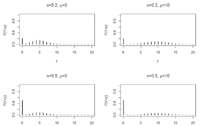
Plot the PMF and CDF for a ZIP distribution with parameters: π = 0.25 and λ = 3. Set the range of count values from 0 to 10.

Exercise 4: Probabilities from CDF

For a ZIP distribution with π = 0.4 and λ = 5, find the probability that Y is less than or equal to 3, i.e., P(Y ≤ 3).

Exercise 5: Expected Value (Mean) from PMF

For a ZIP distribution with π = 0.2 and unknown λ, calculate the expected number of events (mean) using the PMF formula.

Exercise 6: Finding Parameters from PMF

Given the observed PMF values for a ZIP distribution with y = 0, 1, 2, 3, and π = 0.35, determine the Poisson parameter λ using the formula for the ZIP PMF.

Exercise 7: ZIP PMF for Zero Counts

Given π = 0.15 and λ = 4, calculate the probability of observing zero counts (P(Y = 0)) from the ZIP PMF.

Exercise 8: ZIP CDF for Non-Zero Counts

Given π = 0.2 and λ = 3, calculate the cumulative probability of Y being less than or equal to 4 (P(Y ≤ 4 | Y > 0)) from the ZIP CDF.

Exercise 9: Comparison with Poisson Distribution

Compare the ZIP PMF with the Poisson PMF for the same λ (e.g., λ = 2) and observe the differences in probabilities for various count values.

Exercise 10: Data Analysis with ZIP

Analyze a real-world dataset with count data exhibiting zero-inflation. Calculate the PMF and CDF for the dataset using appropriate ZIP distribution parameters.

These exercises will help you gain hands-on experience in working with the PMF and CDF of the ZIP distribution, understand how probabilities change with varying parameters, and interpret the results in practical contexts. Additionally, you can use Python and libraries like scipy.stats or numpy to perform the calculations and create plots for the ZIP PMF and CDF.